21 Taybetmendiyên Kêrhatî yên Excel ji bo Bazirganên Serhêl

Internet marketing is an incredibly lucrative field of human activity, especially in recent times, when any business is moving online whenever possible. And despite the fact that many business processes are managed by specialized programs, a person does not always have enough budget to acquire them, as well as time to master them.

And the solution to this problem is very simple – good old Excel, in which you can maintain lead databases, mailing lists, analyze marketing performance, plan a budget, conduct research and perform other necessary operations in this difficult task. Today we will get acquainted with 21 Excel functions that will suit every Internet marketer. Before we start, let’s understand some key concepts:

1. Syntax. These are the constituent parts of the function and how it is written and in what sequence these components are built. In general, the syntax of any function is divided into two parts: its name itself and arguments – those variables that the function accepts in order to get a result or perform a certain action. Before you write a formula, you need to put an equal sign, which in Excel denotes the character of its input.
2. Arguments can be written in both numeric and text format. Moreover, you can use other operators as arguments, which allows you to write full-fledged algorithms in Excel. An argument that has taken a value is called a function parameter. But very often these two words are used as synonyms. But in fact, there is a difference between them. An argument block begins with an open bracket, separated by a semicolon, and an argument block ends with a closed bracket.

Ready function example − =SUM(A1:A5). Well, shall we begin?

Fonksiyona VLOOKUP

With this feature, the user can find information that matches certain criteria and use it in another formula or write it in a different cell. VPR is an abbreviation that stands for “Vertical View”. This is a fairly complex formula that has four arguments:

1. The desired value. This is the value by which the search for the information that we will need will be carried out. It serves as the address of a cell or value either on its own or returned by another formula.
2. Table. This is the range where you need to search for information. The required value must be in the first column of the table. The return value can be absolutely in any cell that is included in this range.
3. Column number. This is the ordinal number (attention – not the address, but the ordinal number) of the column that contains the value.
4. Interval viewing. This is a boolean value (that is, here you need to enter the formula or value that produces RAST or DEREWAN), which indicates how structured the information should be. If you pass this argument a value RAST, then the contents of the cells must be ordered in one of two ways: alphabetically or ascending. In this case, the formula will find the value that is most similar to the one being searched for. If you specify as an argument DEREWAN, then only the exact value will be searched. In this situation, the sorting of the column data is not so important.

The last argument is not so important to use. Let’s give some examples of how this function can be used. Suppose we have a table that describes the number of clicks for different queries. We need to find out how many were carried out for the request “buy a tablet”.

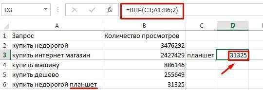
In our formula, we were looking exclusively for the word “tablet”, which we set as the desired value. The “table” argument here is a set of cells that begins with cell A1 and ends with cell B6. The column number in our case is 2. After we entered all the necessary parameters into the formula, we got the following line: =VLOOKUP(C3;A1:B6;2).

After we wrote it into the cell, we got a result corresponding to the number of requests to buy a tablet. You can see it in the screenshot above. In our case, we used the function VPR with different indications of the fourth argument.

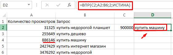
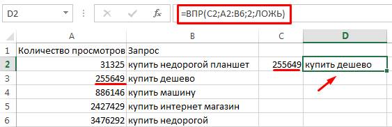
Here we entered the number 900000, and the formula automatically found the closest value to this and issued the query “buy a car”. As we can see, the “interval lookup” argument contains the value RAST. If we search with the same argument that is FALSE, then we need to write the exact number as the search value, as in this screenshot.

Wekî ku em dibînin, fonksiyonek VPR has the broadest possibilities, but it is, of course, difficult to understand. But the gods did not burn the pots.

IF function

This function is needed in order to add some programming elements to the spreadsheet. It allows the user to check if a variable meets certain criteria. If yes, then the function performs one action, if not, another. The syntax for this function includes the following arguments:

1. Direct boolean expression. This is the criterion that must be checked. For example, whether the weather outside is below zero or not.
2. The data to process if the criterion is true. The format can be not only numeric. You can also write a text string that will be returned to another formula or written to a cell. Also, if the value is true, you can use a formula that will perform additional calculations. You can also use functions GER, which are written as arguments to another function IF. In this case, we can set a full-fledged algorithm: if the criterion meets the condition, then we perform action 1, if it does not, then we check for compliance with criterion 2. In turn, there is also branching. If there are a lot of such chains, then the user can get confused. Therefore, it is still recommended to use macros to write complex algorithms.
3. Value if false. This is the same only if the expression does not match the criteria given in the first argument. In this case, you can use exactly the same arguments as in the previous case.

To illustrate, let’s take a small example.

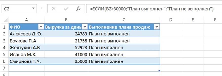
The formula shown in this screenshot checks if the daily revenue is greater than 30000. If yes, then the cell displays information that the plan was completed. If this value is less than or equal, then a notification is displayed that the plan was not completed. Note that we always enclose text strings in quotes. The same rule applies to all other formulas. Now let’s give an example showing how to use multiple nested functions IF.

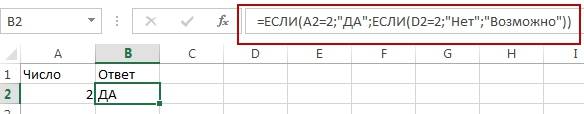
We see that there are three possible results of using this formula. Maximum number of results that a formula with nested functions is limited to IF - 64. You can also check if a cell is empty. To perform this type of check, there is a special formula called EPUSTO. It allows you to replace a long function IF, which checks if the cell is empty, with one simple formula. In this case, the formula will be:

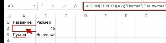Karî ISBLANK returns takes a cell as an argument, and always returns a boolean value. Function IF is at the core of a lot of other features that we’re going to look at next, because they play such a big role in marketing. In fact, there are a lot of them, but we will look at three today: SUMMESLI, COUNTIF, IFERROR.

SUMIF and SUMIFS functions

Karî SUMMESLI makes it possible to sum only those data that meet a certain criterion and are in the range. This function has three arguments:

1. Range. This is a set of cells that needs to be checked to see if there are any cells among it that match the specified criterion.
2. Criterion. This is an argument that specifies the exact parameters under which the cells will be summed. Any type of data can serve as a criterion: cell, text, number, and even a function (for example, a logical one). It is important to consider that criteria containing text and mathematical symbols must be written in quotation marks.
3. Summation range. This argument does not need to be specified if the summation range is the same as the range to test the criterion.

Let’s take a small example to illustrate. Here, using the function, we added up all requests that have more than one hundred thousand transitions.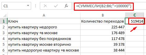

There is also a second version of this function, which is written as SUMMESLIMN. With its help, several criteria can be taken into account at once. Its syntax is flexible and depends on the number of arguments to be used. The generic formula looks like this: =SUMIFS(summation_range, condition_range1, condition1, [condition_range2, condition2], …). The first three arguments must be specified, and then everything depends on how many criteria the person wants to set.

COUNTIF and COUNTIFS functions

This function determines how many cells in a range that match a certain condition. The function syntax includes the following arguments:

1. Range. This is the dataset that will be validated and counted.
2. Criterion. This is the condition that the data must meet.

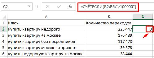
In the example we are giving now, this function determined how many keys with more than one hundred thousand transitions. It turned out that there were only three such keys.

The maximum possible number of criteria in this function is one condition. But similarly to the previous option, you can use the function COUNTIFSto set more criteria. The syntax for this function is: COUNTIFS(condition_range1, condition1, [condition_range2, condition2], …).

The maximum number of conditions and ranges to be checked and calculated is 127.

fonksiyona ERROR

With this function, the cell will return a user-specified value if an error occurs as a result of the calculation for a certain function. The syntax of this function is as follows: =IFERROR(nirx;nirx_eger_çewtî). As you can see, this function requires two arguments:

1. Meaning. Here you need to write down the formula, according to which errors will be processed, if any.
2. The value if an error. This is the value that will be displayed in the cell if the formula operation fails.

And an example to illustrate. Suppose we have such a table.

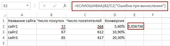
We see that the counter does not work here, so there are no visitors, and 32 purchases were made. Naturally, such a situation cannot happen in real life, so we need to process this error. We did just that. We scored in a function IFERROR argument in the form of a formula for dividing the number of purchases by the number of visitors. And if an error occurs (and in this case it is division by zero), the formula writes “recheck”. This function knows that division by zero is not possible, so it returns the appropriate value.

LEFT function

With this function, the user can get the desired number of characters of the text string, which are located on the left side. The function contains two arguments. In general, the formula is as follows: =LEFT(text,[number_of_characters]).

The arguments to this function include a text string or cell that contains the characters to be retrieved, as well as the number of characters to be counted from the left side. In marketing, this feature will allow you to understand how titles to web pages will look like.

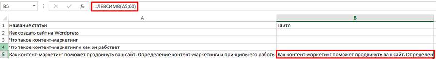
In this case, we have selected 60 characters from the left of the string contained in cell A5. We wanted to test how a concise title would look like.

PTR function

This function is actually similar to the previous one, only it allows you to select a starting point from which to start counting characters. Its syntax includes three arguments:

1. Text string. Purely theoretically, you can write a line here directly, but it is much more efficient to give links to cells.
2. Starting position. This is the character from which the count of the number of characters that are described in the third argument starts.
3. Number of characters. An argument similar to the one in the previous function.

With this function, for example, you can remove a certain number of characters at the beginning and end of a text string.

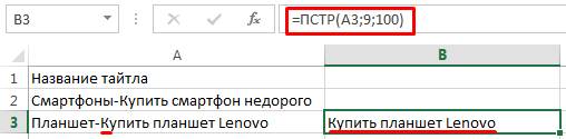
In our case, we removed them only from the beginning.

fonksiyona UPPER

If you need to make sure that all words in a text string located in a specific cell are written in capital letters, then you can use the function RULNTVAN. It takes only one argument, a text string to be made large. It can be either directly hammered into a bracket, or into a cell. In the latter case, you must provide a link to it.

LOWER function

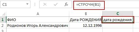
This function is the exact opposite of the previous one. With its help, you can make all the letters in the string be small. It also takes just one argument as a text string, either expressed directly as text or stored in a specific cell. Here’s an example of how we used this function to change the name of the “Date of Birth” column to one where all letters are small.

fonksiyona SEARCH

With this function, the user can determine the presence of a certain element in the value set and understand exactly where it is located. Contains several arguments:

1. The desired value. This is the text string, the number, that should be searched for in the data range.
2. The array being viewed. The set of data that is searched to find the value contained in the previous argument.
3. Mapping type. This argument is optional. With it, you can find the data more accurately. There are three types of comparison: 1 – value less than or equal (we are talking about numeric data, and the array itself must be sorted in ascending order), 2 – exact match, -1 – value greater than or equal.

For clarity, a small example. Here we tried to understand which of the requests has a number of transitions less than or equal to 900.

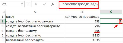
The formula returned the value 3, which is not an absolute row number, but a relative one. That is, not by an address, but by a number relative to the beginning of the selected data range, which can start anywhere.

DLSTR function

This function makes it possible to calculate the length of a text string. It takes one argument – the address of the cell or a text string. For example, in marketing, it is good to use it to check the number of characters in the description.

fonksiyona CONCATENATE

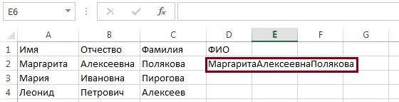
With this operator, you can concatenate multiple text values ​​into one large string. The arguments are cells or directly text strings in quotation marks separated by commas. And here is a small example of using this function.

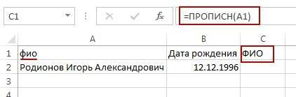
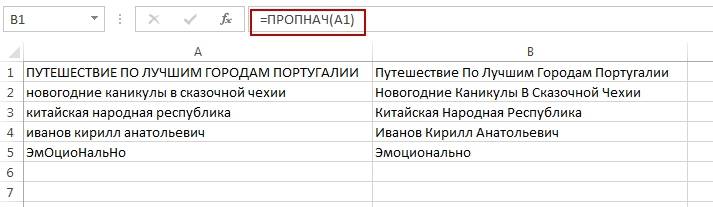
Function PROP

This operator allows you to make all the first letters of words begin in capitals. It takes a text string or a function that returns one as its only argument. This function is well suited for writing lists that include many proper names or other situations where it can be useful.

FUNCTION FUNCTION

This operator makes it possible to remove all invisible characters from a text string. Takes only one argument. In this example, the text contains a non-printable character that was removed by the function.

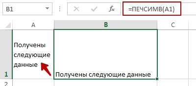
This feature should be used in situations where the user has copied text from another program and non-printable characters have been automatically transferred to an Excel spreadsheet.

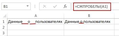
fonksiyona TRIM

With this operator, the user can remove all unnecessary spaces between words. Includes the address of the cell, which is the only argument. Here is an example of using this function to leave only one space between words.

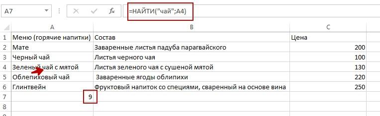
fonksiyona FIND

With this function, the user can find text inside other text. This function is case sensitive. Therefore, large and small characters must be respected. This function takes three arguments:

1. The desired text. This is the string that is being searched for.
2. The text being looked up is the range in which the search is performed.
3. Start position is an optional argument that specifies the first character from which to search.

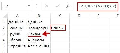
fonksiyona INDEX

With this function, the user can get the value he is looking for. It has three required arguments:

1. Array. The range of data being analyzed.
2. Line number. The ordinal number of the row in this range. Attention! Not an address, but a line number.
3. Column number. Same as the previous argument, only for the column. This argument can be left blank.

fonksiyona EXACT

This operator can be used to determine if two text strings are the same. If they are identical, it returns the value RAST. If they are different – DEREWAN.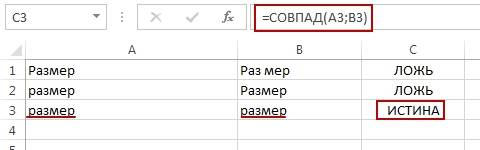

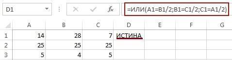
OR fonksiyona

This function allows you to set the choice of condition 1 or condition 2. If at least one of them is true, then the return value is – RAST. You can specify up to 255 boolean values.

Fonksiyon Û

The function returns a value RASTif all of its arguments return the same value.

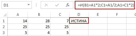
This is the most important logical argument that allows you to set several conditions at once, which must be simultaneously observed.

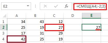
fonksiyona OFFSET

This function allows you to get a reference to a range that is offset by a certain number of rows and columns from the original coordinates. Arguments: reference to the first cell of the range, how many rows to shift, how many columns to shift, what is the height of the new range and what is the width of the new range.

Xelasî

With the help of Excel functions, a marketer can more flexibly analyze site performance, conversion, and other indicators. As you can see, no special programs are required, the good old office suite is enough to implement almost any idea.