Meriv çawa di Excel de navnîşek dakêşanê çêdike. Bi navgîniya pêşek û amûrên pêşdebir re

Numerous Excel users, who often use this program, work with a lot of data that constantly needs to be entered over a large number of times. A drop-down list will help to facilitate the task, which will eliminate the need for constant data entry.

Create a dropdown list using the context menu

This method is simple and after reading the instructions it will be clear even to a beginner.

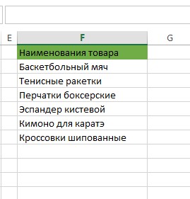
1. First you need to create a separate list in any area of ​​uXNUMXbuXNUMXbthe sheet. Or, if you don’t want to litter the document so you can edit it later, create a list on a separate sheet.
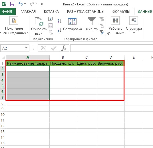
2. Having determined the boundaries of the temporary table, we enter a list of product names into it. Each cell should contain only one name. As a result, you should get a list executed in a column.
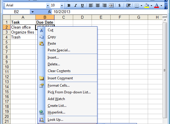
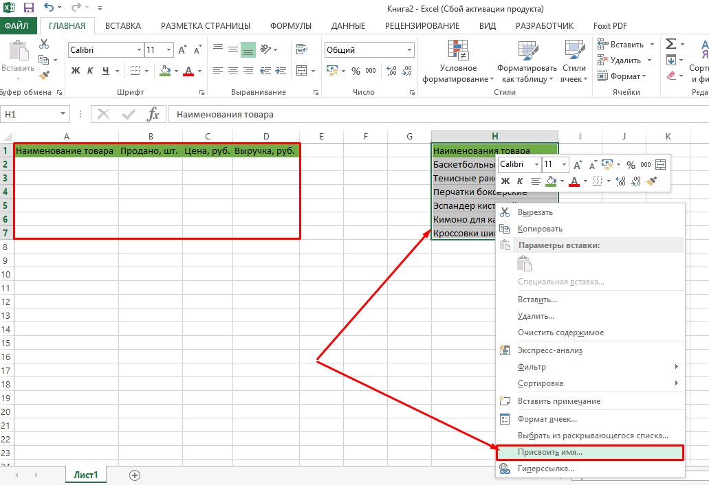
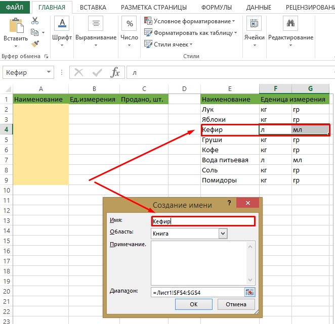
3. Having selected the auxiliary table, right-click on it. In the context menu that opens, go down, find the item “Assign a name …” and click on it.

4. A window should appear where, opposite the “Name” item, you must enter the name of the created list. Once the name is entered, click the “OK” button.

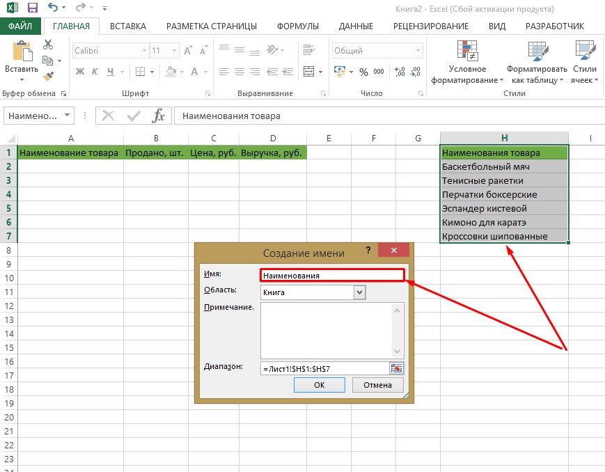
Giring! When creating a name for a list, you need to take into account a number of requirements: the name must begin with a letter (space, symbol or number are not allowed); if several words are used in the name, then there should not be spaces between them (as a rule, an underscore is used). In some cases, to facilitate the subsequent search for the required list, users leave notes in the “Note” item.

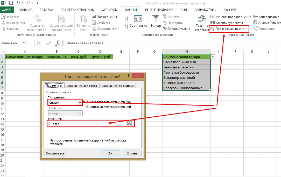
5. Select the list you want to edit. At the top of the toolbar in the “Work with data” section, click on the “Data Validation” item.
6. In the menu that opens, in the “Data Type” item, click on “List”. We go down and enter the “=” sign and the name given earlier to our auxiliary list (“Product”). You can agree by clicking the “OK” button.

5. The work can be considered completed. After clicking on each of the cells, a special icon should appear on the left with an embedded triangle, one corner of which looks down. This is an interactive button that, when clicked, opens a list of previously compiled items. It remains only to click to open the list and enter a name in the cell.

Şîreta pispor! Thanks to this method, you can create the entire list of goods available in the warehouse and save it. If necessary, it remains only to create a new table in which you will need to enter the names that currently need to be accounted for or edited.

Building a List Using Developer Tools

The method described above is far from the only method for creating a drop-down list. You can also turn to the help of developer tools to complete this task. Unlike the previous one, this method is more complex, which is why it is less popular, although in some cases it is considered an indispensable help from the accountant.

To create a list in this way, you need to face a large set of tools and perform many operations. Although the end result is more impressive: it is possible to edit the appearance, create the required number of cells and use other useful features. Let’s get started:

1. First you need to connect the developer tools, as they may not be active by default.
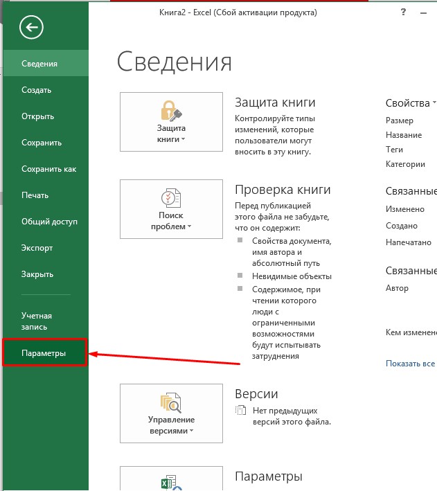
2. To do this, open “File” and select “Options”.

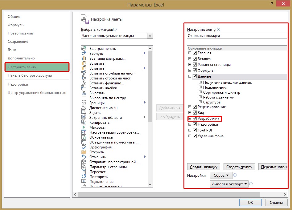
3. A window will open, where in the list on the left we look for “Customize Ribbon”. Click and open the menu.
4. In the right column, you need to find the item “Developer” and put a checkmark in front of it, if there was none. After that, the tools should be automatically added to the panel.

5. Ji bo tomarkirina mîhengan, bişkojka "OK" bikirtînin.
6. With the advent of the new tab in Excel, there are many new features. All further work will be performed using this tool.
7. Next, we create a list with a list of product names that will pop up if you need to edit a new table and enter data into it.

8. Activate the developer tool. Find “Controls” and click on “Paste”. A list of icons will open, hovering over them will display the functions they perform. We find the “Combo Box”, it is located in the “ActiveX Controls” block, and click on the icon. The “Designer Mode” should turn on.

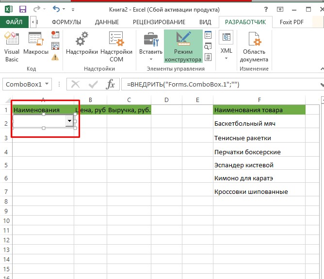
9. Having selected the top cell in the prepared table, in which the list will be placed, we activate it by clicking LMB. Set up its boundaries.
10. The selected list activates “Design Mode”. Nearby you can find the “Properties” button. It must be enabled to continue customizing the list.
11. The options will open. We find the line “ListFillRange” and enter the addressing of the auxiliary list.
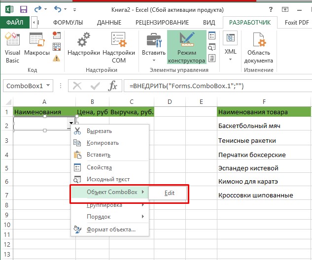
12. RMB click on the cell, in the menu that opens, go down to “ComboBox Object” and select “Edit”.

9. Mission

Not! In order for the list to display several cells with a drop-down list, it is necessary that the area near the left edge, where the selection marker is located, remain open. Only in this case is it possible to capture the marker.

Creating a linked list

You can also create linked lists to make your work easier in Excel. Let’s figure out what it is and how to make them in the simplest way.

1. We create a table with a list of product names and their units of measurement (two options). To do this, you need to make at least 3 columns.

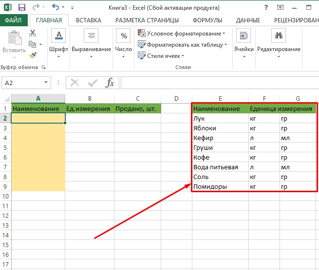
2. Next, you need to save the list with the names of the products and give it a name. To do this, having selected the column “Names”, right-click and click “Assign a name.” In our case, it will be “Food_Products”.
3. Similarly, you need to generate a list of units of measure for each name of each product. We complete the entire list.

4. Activate the top cell of the future list in the “Names” column.
5. Through working with data, click on data verification. In the drop-down window, select “List” and below we write the assigned name for the “Name”.
6. In the same way, click on the top cell in units of measure and open the “Check Input Values”. In the paragraph “Source” we write the formula: =INDIRECT(A2).
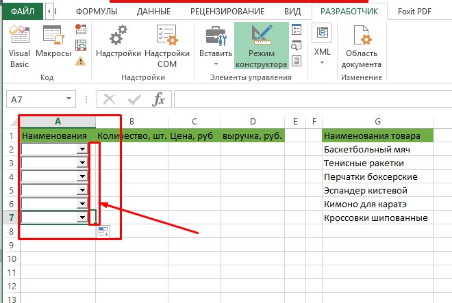
7. Next, you need to apply the autocomplete token.
8. Ready! You can start filling in the table.

Xelasî

Drop-down lists in Excel are a great way to make working with data easier. The first acquaintance with the methods of creating drop-down lists may suggest the complexity of the process being performed, but this is not the case. This is just an illusion that is easily overcome after a few days of practice according to the above instructions.