Meriv çawa di Excel de forma hucreyê biguhezîne. Bi navgîniya menuya çarçoveyê, amûr û bişkojkên germ

Each of the cells has its own format that allows you to process information in one form or another. It is important to set it correctly so that all the necessary calculations are carried out correctly. From the article you will learn how to change the format of cells in an Excel spreadsheet.

The main types of formatting and their change

There are ten basic formats in total:

1. Hevre.
2. Monetary.
3. Numerical.
4. Aborî.
5. Nivîstok.
6. Rojek.
7. Dem.
8. Biçûk.
9. Percentage.
10. Biserre

Some formats have their own additional subspecies. There are several methods to change the format. Let’s analyze each in more detail.

Rêbaz 1: menuya çarçoveyê

Using the context menu to edit a format is one of the most commonly used methods. Rêwîtî:

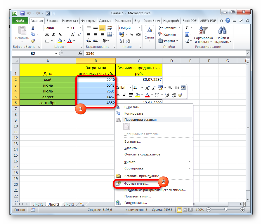
1. You need to select those cells whose format you want to edit. We click on them with the right mouse button. A special context menu has opened. Click on the element “Format Cells …”.

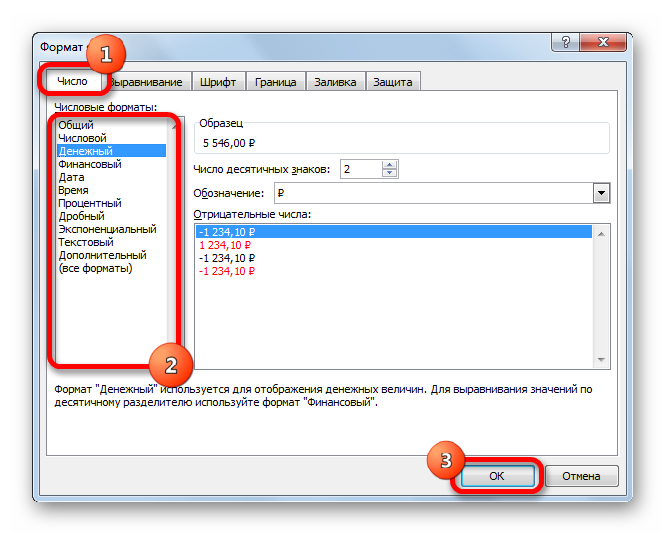
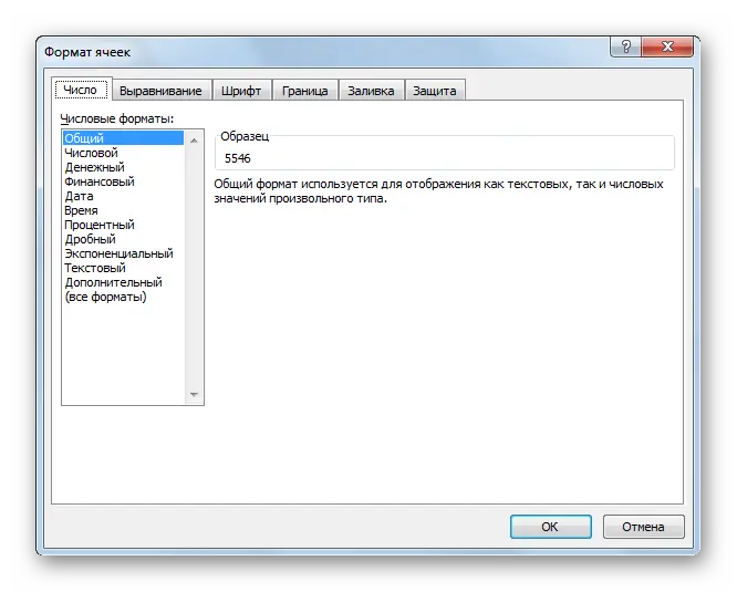
2. A format box will appear on the screen. We move to the section called “Number”. Pay attention to the block “Number formats”. Here are all the existing formats that were given above. We click on the format that corresponds to the type of information that is given in the cell or range of cells. To the right of the format block is the subview setting. After making all the settings, click “OK”.

3. Ready. Format editing was successful.

Method 2: Number toolbox on the ribbon

The tool ribbon contains special elements that allow you to change the format of cells. Using this method is much faster than the previous one. Walkthrough:

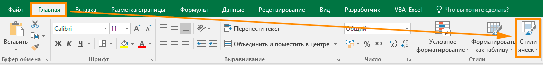
1. We carry out the transition to the section “Home”. Next, select the desired cell or range of cells and open the selection box in the “Number” block.

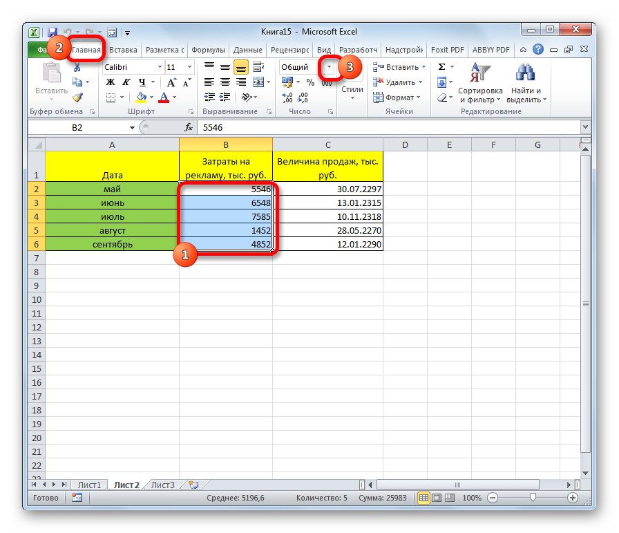
2. The main format options were revealed. Choose the one you need in the selected area. The formatting has changed.

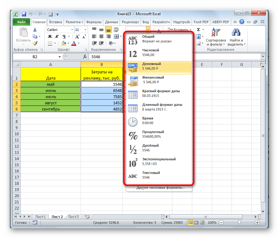
3. It should be understood that this list contains only the main formats. In order to expand the entire list, you need to click “Other number formats”.

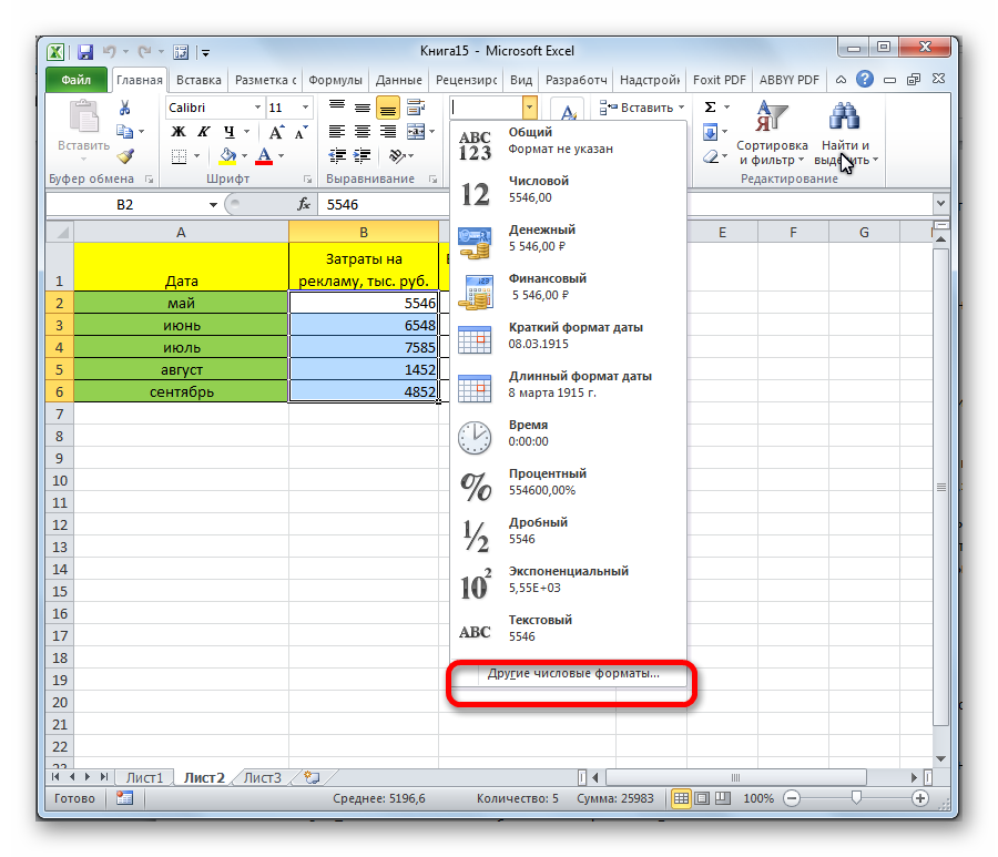
4. After clicking on this element, a familiar window will appear with all possible formatting options (basic and additional).

Method 3: “Cells” toolbox

The next format editing method is performed through the “Cells” block. Walkthrough:

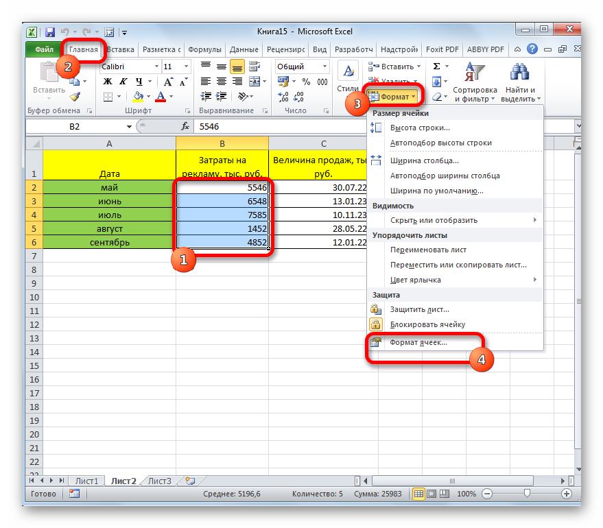
1. We select the cell or range of cells whose format we want to change. We move to the “Home” section, click on the inscription “Format”. This element is located in the “Cells” block. In the drop-down list, click on “Format Cells …”.

2. After this action, the usual formatting window appeared. We perform all the necessary actions, choosing the desired format and clicking “OK”.

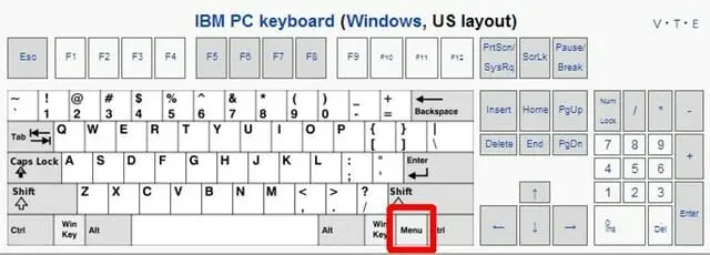
Rêbaz 4: bişkojkên germ

The cell format can be edited using special spreadsheet hotkeys. First you need to select the desired cells, and then press the key combination Ctrl + 1. After the manipulations, the familiar format change window will open. As in the previous methods, select the desired format and click “OK”. Additionally, there are other keyboard shortcuts that allow you to edit the cell format without displaying the format box:

• Ctrl+Shift+- – general.
• Ctrl+Shift+1 — numbers with a comma.
• Ctrl+Shift+2 – time.
• Ctrl+Shift+3 — date.
• Ctrl+Shift+4 – money.
• Ctrl+Shift+5 – percentage.
• Ctrl+Shift+6 – O.OOE+00 format.

Date format with time in Excel and 2 display systems

The date format can be further formatted using spreadsheet tools. For example, we have this tablet with information. We need to make sure that the indicators in the rows are brought to the form indicated in the column names.

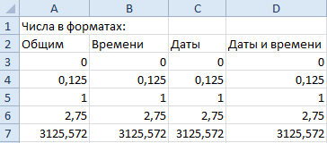
In the first column, the format is initially set correctly. Let’s look at the second column. Select all cells of indicators of the second column, press the key combination CTRL + 1, in the “Number” section, select the time, and in the “Type” tab, select the display method corresponding to the following picture:

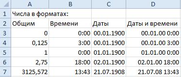
We carry out similar actions with the third and fourth columns. We set those formats and display types that correspond to the declared column names. There are 2 date display systems in the spreadsheet:

1. The number 1 is January 1, 1900.
2. The number 0 is January 1, 1904, and the number 1 is 02.01.1904/XNUMX/XNUMX.

Changing the display of dates is carried out as follows:

1. Let’s go to “File”.
2. Click “Options” and move to the “Advanced” section.
3. In the “When recalculating this book” block, select the “Use the 1904 date system” option.

Alignment Tab

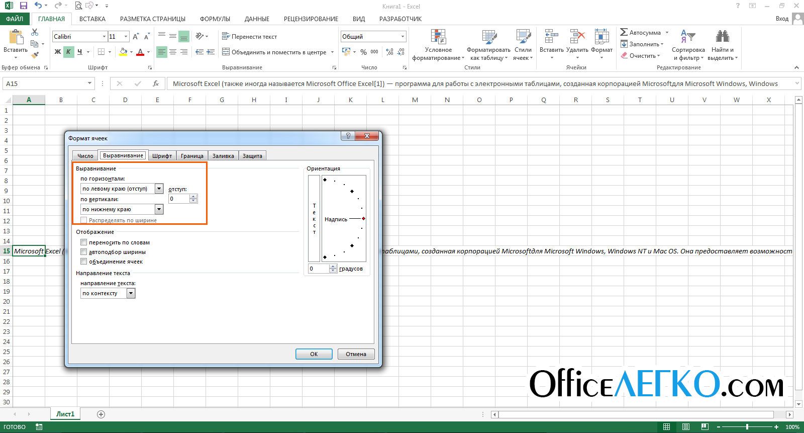
Using the “Alignment” tab, you can set the location of the value inside the cell by several parameters:

• towards;
• horizontally;
• vertically;
• relative to the center;
• wate ya vê çîye.

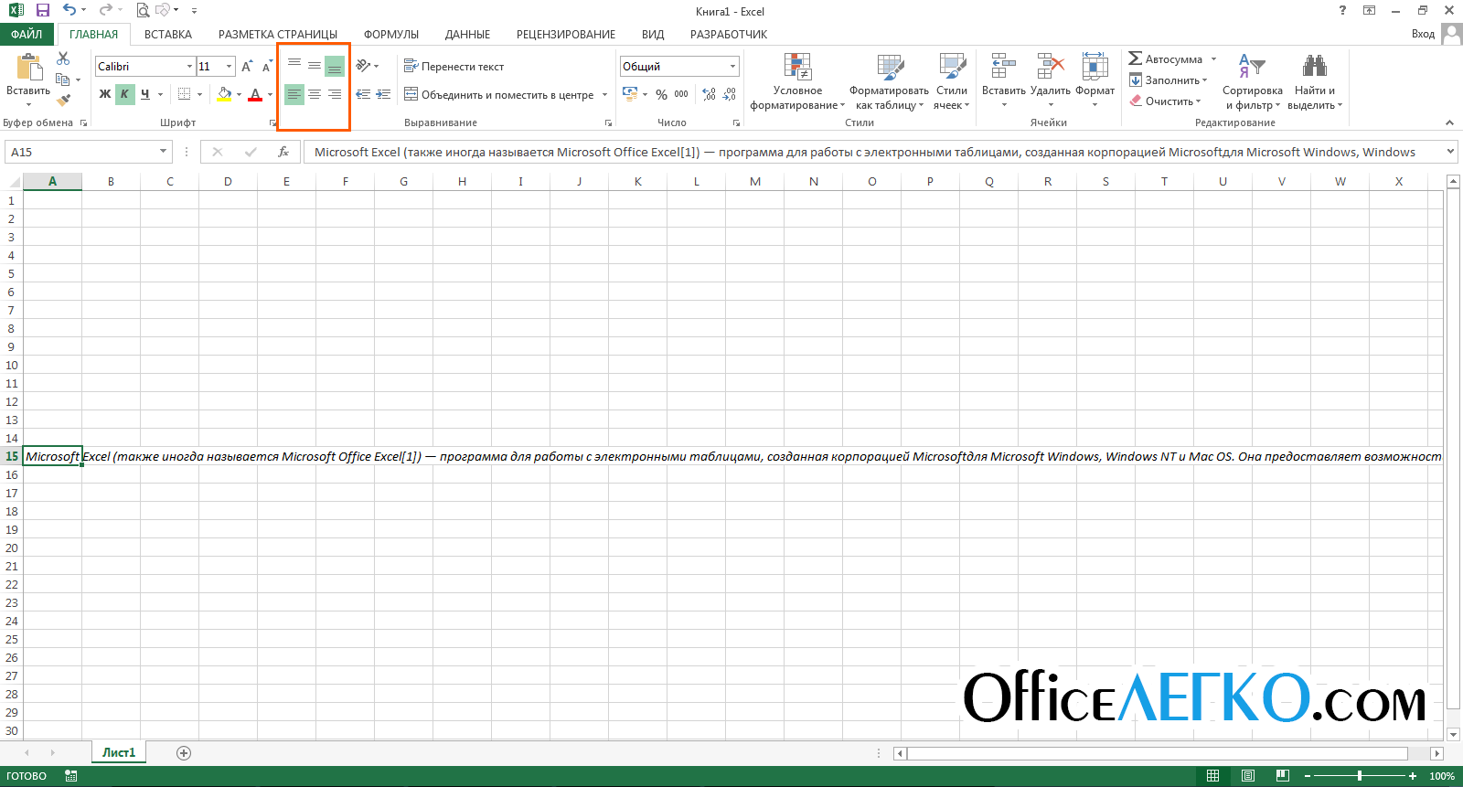
By default, the typed number in the cell is right-aligned, and text information is left-aligned. In the “Alignment” block, the “Home” tab, you can find the basic formatting elements.

With the help of ribbon elements, you can edit the font, set borders and change the fill. You just need to select a cell or a range of cells and use the top toolbar to set all the desired settings.

I am editing the text

Let’s look at several ways to customize the text in the cells to make tables with information as readable as possible.

How to change the Excel font

Let’s look at several ways to change the font:

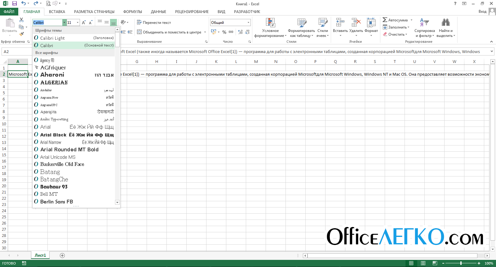
1. Method one. Select the cell, go to the “Home” section and select the “Font” element. A list opens in which each user can choose the appropriate font for themselves.

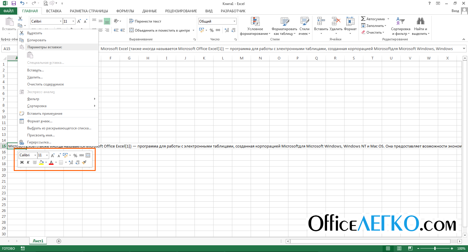
2. Method two. Select a cell, right-click on it. A context menu is displayed, and below it is a small window that allows you to format the font.

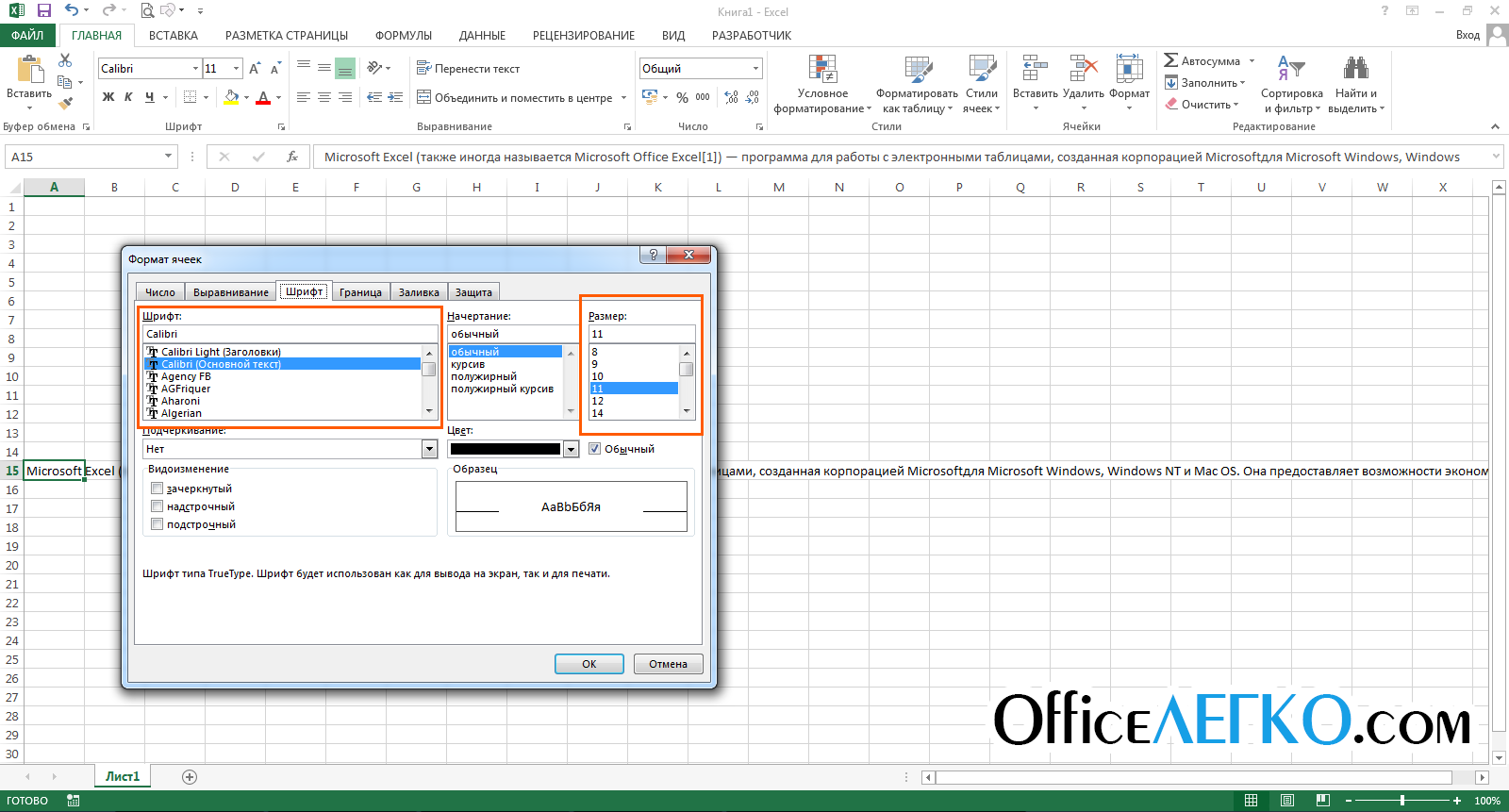
3. Method three. Select the cell and use the key combination Ctrl + 1 to call “Format Cells”. In the window that appears, select the “Font” section and make all the necessary settings.

How to Choose Excel Styles

Bold, italic, and underline styles are used to highlight important information in tables. To change the style of the entire cell, you need to click on it with the left mouse button. To change only part of a cell, you need to double-click on the cell, and then select the desired part for formatting. After selection, change the style using one of the following methods:

1. Using key combinations:

• Ctrl+B – bold;
• Ctrl+I – italic;
• Ctrl+U – underlined;
• Ctrl + 5 – crossed out;
• Ctrl+= – subscript;
• Ctrl+Shift++ – superscript.

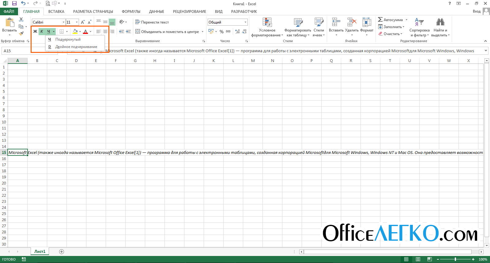
2. Using the tools located in the “Font” block of the “Home” tab.

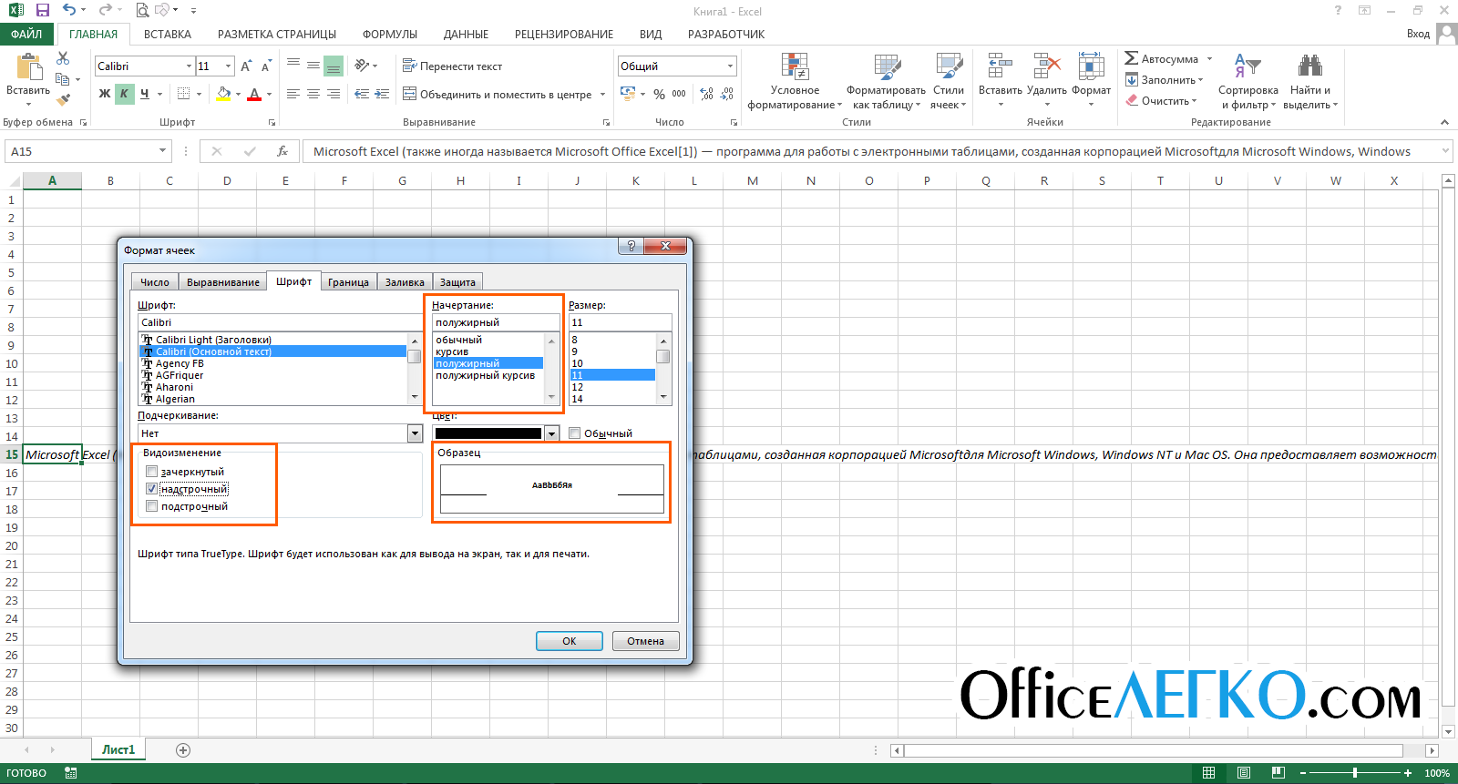
3. Using the Format Cells box. Here you can set the desired settings in the “Modify” and “Inscription” sections.

Aligning text in cells

Alignment of text in cells is carried out by the following methods:

• Go to the “Alignment” section of the “Home” section. Here, with the help of icons, you can align the data.

• In the “Format Cells” box, go to the “Alignment” section. Here you can also select all existing types of alignment.

Auto-format text in Excel

Balkêşandin! Long text entered into a cell may not fit in it and then it will be displayed incorrectly. There is an auto-formatting feature to avoid this problem.

Two methods of autoformatting:

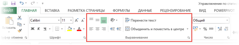
1. Applying word wrap. Select the desired cells, go to the “Home” section, then to the “Alignment” block and select “Move Text”. Enabling this feature allows you to automatically implement word wrapping and increase the line height.
2. Using the AutoFit function. Go to the “Format Cells” box, then “Alignment” and check the box next to “AutoFit Width”.

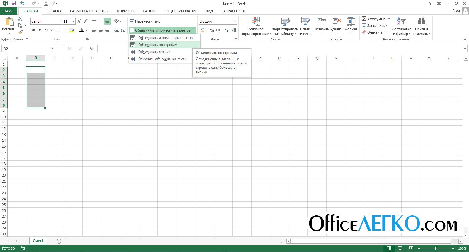
How to merge cells in Excel

Often, when working with tables, it becomes necessary to merge cells. This can be done using the “Merge and Center” button, which is located in the “Alignment” block of the “Home” section. Using this option will merge all selected cells. Values ​​inside cells are aligned to the center.

Changing the Orientation and Direction of Text

Text direction and orientation are two different settings that some users confuse with each other. In this figure, the first column uses the orientation function, and the second column uses the direction:

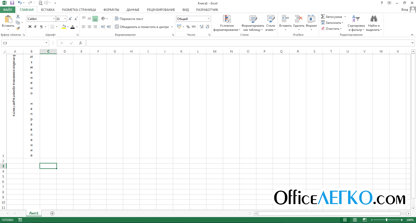
By going to the “Home” section, the “Alignment” block and the “Orientation” element, you can apply these two parameters.

Working with Excel Cell Formatting Styles

Using formatting styles can significantly speed up the process of formatting a table and give it a beautiful appearance.

Why Named Styles Are Necessary

The main purposes of using styles:

1. Create unique style sets for editing headings, subheadings, text, and more.
2. Applying created styles.
3. Automation of work with data, since using the style, you can format absolutely all data in the selected range.

Applying styles to worksheet cells

There are a huge number of integrated ready-made styles in the spreadsheet processor. Step by step guide to use styles:

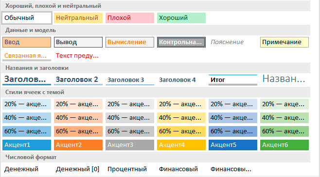
1. Go to the “Home” tab, find the “Cell Styles” block.

2. The library of ready styles is displayed on the screen.
3. Select the desired cell and click on the style you like.
4. The style has been applied to the cell. If you just hover your mouse over a suggested style, but don’t click on it, you can preview how it will look.

Creating New Styles

Often, users do not have enough ready-made styles, and they resort to developing their own. You can make your own unique style as follows:

1. Select any cell and format it. We will create a style based on this formatting.
2. Go to the “Home” section and move to the “Cell Styles” block. Click “Create Cell Style”. A window called “Style” opens.

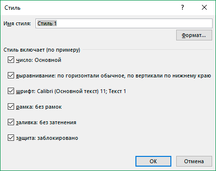
3. Enter any “Style Name”.
4. We set all the necessary parameters that you want to apply to the created style.
5. We click “OK”.
6. Now your unique style has been added to the style library, which can be used in this document.

Changing Existing Styles

Ready-made styles located in the library can be changed independently. Walkthrough:

1. Go to the “Home” section and select “Cell Styles”.
2. Right-click on the style you want to edit and click Edit.
3. The Style window opens.
4. Click “Format” and in the displayed window “Format Cells” adjust the formatting. After carrying out all the manipulations, click “OK”.
5. Click OK again to close the Style box. Editing of the finished style is completed, now it can be applied to document elements.

Transferring Styles to Another Book

Giring! A created style can only be used in the document in which it was created, but there is a special feature that allows you to transfer styles to other documents.

Rêwîtî:

1. We tear off the document in which the created styles are located.
2. Additionally, open another document into which we want to transfer the created style.
3. In the document with styles, go to the “Home” tab and find the “Cell Styles” block.
4. Click “Combine”. A window called “Merge Styles” appeared.
5. This window contains a list of all open spreadsheet documents. Select the document to which you want to transfer the created style and click the “OK” button. Ready!

Xelasî

There are a huge number of methods that allow you to edit the cell format in a spreadsheet. Thanks to this, each person working in the program can choose for himself a more convenient way to solve certain problems.