


Contents
Congratulations! You made it to the final day of the marathon 30 fonksiyonên Excel di 30 rojan de. It has been a long and interesting journey during which you have learned many useful things about Excel functions.
Di roja 30emîn a maratonê de, em ê lêkolîna fonksiyonê bikin NADIREKT (INDIRECT), which returns the link specified by the text string. With this function, you can create dependent drop-down lists. For example, when selecting a country from a dropdown list determines which options will appear in the city dropdown list.
So, let’s take a closer look at the theoretical part of the function NADIREKT (INDIRECT) and explore practical examples of its application. If you have additional information or examples, please share them in the comments.
Function 30: INDIRECT
Karî NADIREKT (NEDIREKT) lînka ku bi rêzika nivîsê hatiye diyarkirin vedigerîne.
How can you use the INDIRECT function?
Ji ber ku fonksiyonê NADIREKT (INDIRECT) returns a link given by a text string, you can use it to:
- Create a non-shifting initial link.
- Create a reference to a static named range.
- Create a link using sheet, row, and column information.
- Create a non-shifting array of numbers.
Syntax INDIRECT (INDIRECT)
Karî NADIREKT (INDIRECT) has the following syntax:
INDIRECT(ref_text,a1)
ДВССЫЛ(ссылка_на_ячейку;a1)
- ref_text (link_to_cell) is the text of the link.
- a1 – if equal to TRUE (TRUE) or not specified, then the style of the link will be used A1; and if FALSE (FALSE), then the style R1C1.
Traps INDIRECT (INDIRECT)
- Karî NADIREKT (INDIRECT) is recalculated whenever the values in the Excel worksheet change. This can greatly slow down your workbook if the function is used in many formulas.
- Ger fonksiyona NADIREKT (INDIRECT) creates a link to another Excel workbook, that workbook must be open or the formula will report an error #REF! (#PÊVEK!).
- Ger fonksiyona NADIREKT (INDIRECT) references a range that exceeds the row and column limit, the formula will report an error #REF! (#PÊVEK!).
- Karî NADIREKT (INDIRECT) cannot reference a dynamic named range.
Example 1: Create a non-shifting initial link
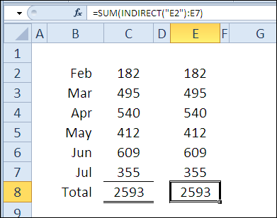
In the first example, columns C and E contain the same numbers, their sums calculated using the function GIŞ (SUM) are also the same. However, the formulas are slightly different. In cell C8, the formula is:
=SUM(C2:C7)
=СУММ(C2:C7)
In cell E8, the function NADIREKT (INDIRECT) creates a link to the starting cell E2:
=SUM(INDIRECT("E2"):E7)
=СУММ(ДВССЫЛ("E2"):E7)
If you insert a row at the top of the sheet and add the value for January (Jan), then the amount in column C will not change. The formula will change, reacting to the addition of a line:
=SUM(C3:C8)
=СУММ(C3:C8)
However, the function NADIREKT (INDIRECT) fixes E2 as the start cell, so January is automatically included in the calculation of column E totals. The end cell has changed, but the start cell has not been affected.
=SUM(INDIRECT("E2"):E8)
=СУММ(ДВССЫЛ("E2"):E8)
Example 2: Link to a static named range
Karî NADIREKT (INDIRECT) can create a reference to a named range. In this example, the blue cells make up the range NumList. In addition, a dynamic range is also created from the values in column B NumListDyn, depending on the number of numbers in this column.
The sum for both ranges can be calculated by simply giving its name as an argument to the function GIŞ (SUM), as you can see in cells E3 and E4.
=SUM(NumList) или =СУММ(NumList)
=SUM(NumListDyn) или =СУММ(NumListDyn)
Instead of typing a range name into a function GIŞ (SUM), You can refer to the name written in one of the cells of the worksheet. For example, if the name NumList is written in cell D7, then the formula in cell E7 will be like this:
=SUM(INDIRECT(D7))
=СУММ(ДВССЫЛ(D7))
Mixabin fonksiyona NADIREKT (INDIRECT) cannot create a dynamic range reference, so when you copy this formula down into cell E8, you will get an error #REF! (#PÊVEK!).
Example 3: Create a link using sheet, row, and column information
You can easily create a link based on the row and column numbers, as well as using the value FALSE (FALSE) for the second function argument NADIREKT (INDIRECT). This is how the style link is created R1C1. In this example, we additionally added the sheet name to the link – ‘MyLinks’!R2C2
=INDIRECT("'"&B3&"'!R"&C3&"C"&D3,FALSE)
=ДВССЫЛ("'"&B3&"'!R"&C3&"C"&D3;ЛОЖЬ)
Example 4: Create a non-shifting array of numbers
Sometimes you need to use an array of numbers in Excel formulas. In the following example, we want to average the 3 largest numbers in column B. The numbers can be entered into a formula, as is done in cell D4:
=AVERAGE(LARGE(B1:B8,{1,2,3}))
=СРЗНАЧ(НАИБОЛЬШИЙ(B1:B8;{1;2;3}))
If you need a larger array, then you are unlikely to want to enter all the numbers in the formula. The second option is to use the function DOR (ROW), as done in the array formula entered in cell D5:
=AVERAGE(LARGE(B1:B8,ROW(1:3)))
=СРЗНАЧ(НАИБОЛЬШИЙ(B1:B8;СТРОКА(1:3)))
The third option is to use the function DOR (STRING) along with NADIREKT (INDIRECT), as done with the array formula in cell D6:
=AVERAGE(LARGE(B1:B8,ROW(INDIRECT("1:3"))))
=СРЗНАЧ(НАИБОЛЬШИЙ(B1:B8;СТРОКА(ДВССЫЛ("1:3"))))
The result for all 3 formulas will be the same:
However, if rows are inserted at the top of the sheet, the second formula will return an incorrect result due to the fact that the references in the formula will change along with the row shift. Now, instead of the average of the three largest numbers, the formula returns the average of the 3rd, 4th, and 5th largest numbers.
Karanîna fonksiyonan NADIREKT (INDIRECT), the third formula keeps the correct row references and continues to show the correct result.