


Contents
Excel is one of the best data analytics software. And almost every person at one stage or another of life had to deal with numbers and text data and process them under tight deadlines. If you still need to do this, then we will describe techniques that will help significantly improve your life. And to make it more visual, we will show how to implement them using animations.
Data Analysis Through Excel PivotTables
Pivot tables are one of the easiest ways to automate information processing. It allows you to pile up a huge array of data that is absolutely not structured. If you use it, you can almost forever forget about what a filter and manual sorting are. And to create them, just press just a couple of buttons and enter a few simple parameters, depending on which way of presenting the results you need specifically in a particular situation.
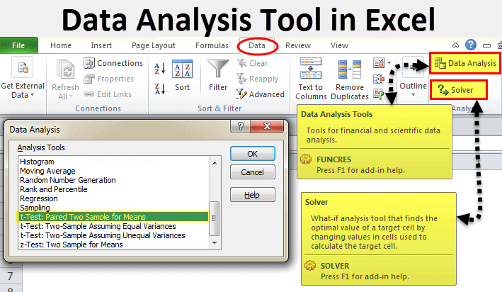
There are many ways to automate data analysis in Excel. These are both built-in tools and add-ons that can be downloaded on the Internet. There is also an add-on “Analysis Toolkit”, which was developed by Microsoft. It has all the necessary features so that you can get all the results you need in one Excel file.
The data analysis package developed by Microsoft can only be used on a single worksheet in one unit of time. If it will process information located on several, then the resulting information will be displayed exclusively on one. In others, ranges will be shown without any values, in which there are only formats. To analyze information on multiple sheets, you need to use this tool separately. This is a very large module that supports a huge number of features, in particular, it allows you to perform the following types of processing:
- Dispersion analysis.
- Correlation analysis.
- Covariance.
- Moving average calculation. A very popular method in statistics and trading.
- Get random numbers.
- Perform selection operations.
This add-on is not activated by default, but is included in the standard package. To use it, you must enable it. To do this, take the following steps:
- Go to the “File” menu, and there find the “Options” button. After that, go to “Add-ons”. If you installed the 2007 version of Excel, then you need to click on the “Excel Options” button, which is located in the Office menu.
- Next, a pop-up menu appears, titled “Management”. There we find the item “Excel Add-ins”, click on it, and then – on the “Go” button. If you are using an Apple computer, then just open the “Tools” tab in the menu, and then find the “Add-ins for Excel” item in the drop-down list.
- In the dialog that appeared after that, you need to check the box next to the “Analysis Package” item, and then confirm your actions by clicking the “OK” button.
In some situations, it may turn out that this add-on could not be found. In this case, it will not be in the list of addons. To do this, click on the “Browse” button. You may also receive information that the package is completely missing from this computer. In this case, you need to install it. To do this, click on the “Yes” button.
Before you can enable the analysis pack, you must first activate VBA. To do this, you need to download it in the same way as the add-on itself.
How to work with pivot tables
The initial information can be anything. This can be information about sales, delivery, shipments of products, and so on. Regardless of this, the sequence of steps will always be the same:
- Open the file containing the table.
- Select the range of cells that we will analyze using the pivot table.
- Open the “Insert” tab, and there you need to find the “Tables” group, where there is a “Pivot Table” button. If you use a computer under the Mac OS operating system, then you need to open the “Data” tab, and this button will be located in the “Analysis” tab.
- This will open a dialog titled “Create PivotTable”.
- Then set the data display to match the selected range.
We have opened a table, the information in which is not structured in any way. To do this, you can use the settings for the fields of the pivot table on the right side of the screen. For example, let’s send the “Amount of orders” in the “Values” field, and information about sellers and the date of sale – in the rows of the table. Based on the data contained in this table, the amounts were automatically determined. If necessary, you can open information for each year, quarter or month. This will allow you to get the detailed information that you need at a particular moment.
The set of available parameters will differ from how many columns there are. For example, the total number of columns is 5. And we just need to place and select them in the right way, and show the sum. In this case, we perform the actions shown in this animation.
You can specify the pivot table by specifying, for example, a country. To do this, we include the “Country” item.
You can also view information about sellers. To do this, we replace the “Country” column with “Seller”. The result will be the following.
Data analysis with 3D maps
This geo-referenced visualization method makes it possible to look for patterns tied to regions, as well as analyze this type of information.
The advantage of this method is that there is no need to separately register the coordinates. You just need to correctly write the geographical location in the table.
How to work with 3D maps in Excel
The sequence of actions that you need to follow in order to work with 3D maps is as follows:
- Open a file that contains the data range of interest. For example, a table where there is a column “Country” or “City”.
- The information that will be shown on the map must first be formatted as a table. To do this, you need to find the corresponding item on the “Home” tab.
- Select the cells to be analyzed.
- After that, go to the “Insert” tab, and there we find the “3D map” button.
Then our map is shown, where the cities in the table are represented as dots. But we don’t really need just the presence of information about settlements on the map. It is much more important for us to see the information that is tied to them. For example, those amounts that can be shown as the height of the column. After we perform the actions indicated in this animation, when you hover over the corresponding column, the data associated with it will be displayed.
You can also use a pie chart, which is much more informative in some cases. The size of the circle depends on what the total amount is.
Forecast sheet in Excel
Often business processes depend on seasonal features. And such factors must be taken into account at the planning stage. There is a special Excel tool for this, which you will like with its high accuracy. It is significantly more functional than all the methods described above, no matter how excellent they may be. In the same way, the scope of its use is very wide – commercial, financial, marketing and even government structures.
Giring: to calculate the forecast, you need to get information for the previous time. The quality of forecasting depends on how long-term the data is. It is recommended to have data that is broken down into regular intervals (for example, quarterly or monthly).
How to work with the forecast sheet
To work with a forecast sheet, you must do the following:
- Open the file, which contains a large amount of information on the indicators that we need to analyze. For example, during the past year (although the more the better).
- Highlight two lines of information.
- Go to the “Data” menu, and there click on the “Forecast Sheet” button.
- After that, a dialog will open in which you can select the type of visual representation of the forecast: a graph or a histogram. Choose the one that suits your situation.
- Set the date when the forecast should end.
In the example below, we provide information for three years – 2011-2013. In this case, it is recommended to indicate time intervals, and not specific numbers. That is, it is better to write March 2013, and not a specific number like March 7, 2013. In order to obtain a forecast for 2014 based on these data, it is necessary to obtain data arranged in rows with the date and indicators that were at that moment. Highlight these lines.
Then go to the “Data” tab and look for the “Forecast” group. After that, go to the “Forecast sheet” menu. After that, a window will appear in which we again select the method for presenting the forecast, and then set the date by which the forecast should be completed. After that, click on “Create”, after which we get three forecast options (shown by an orange line).
Quick analysis in Excel
The previous method is really good because it allows you to make real predictions based on statistical indicators. But this method allows you to actually conduct a full-fledged business intelligence. It is very cool that this feature is created as ergonomically as possible, since in order to achieve the desired result, you need to perform literally a few actions. No manual calculations, no writing down any formulas. Simply select the range to be analyzed and set the end goal.
It is possible to create a variety of charts and micrographs right in the cell.
Meriv çawa dixebite
So, in order to work, we need to open a file that contains the data set that needs to be analyzed and select the appropriate range. After we select it, we will automatically have a button that makes it possible to draw up a summary or perform a set of other actions. It’s called fast analysis. We can also define the amounts that will be automatically entered at the bottom. You can see more clearly how it works in this animation.
The quick analysis feature also allows you to format the resulting data in different ways. And you can determine which values are more or less directly in the cells of the histogram that appears after we configure this tool.
Also, the user can put a variety of markers that indicate larger and smaller values relative to those in the sample. Thus, the largest values will be shown in green, and the smallest ones in red.
I really want to believe that these techniques will allow you to significantly increase the efficiency of your work with spreadsheets and achieve everything you want as quickly as possible. As you can see, this spreadsheet program provides very wide possibilities even in standard functionality. And what can we say about add-ons, which are very numerous on the Internet. It is only important to note that all addons must be carefully checked for viruses, because modules written by other people may contain malicious code. If the add-ons are developed by Microsoft, then it can be safely used.
The Analysis Pack from Microsoft is a very functional add-on that makes the user a true professional. It allows you to perform almost any processing of quantitative data, but it is quite complicated for a novice user. The official Microsoft help site has detailed instructions on how to use different types of analysis with this package.